By Priyank Jain

Introduction:

Machine learning now sits inside telecom operations. Models predict equipment failures before they become outages, forecast traffic for capacity planning, flag telemetry anomalies, and estimate quality of experience from indirect signals—decisions that carry real financial weight. Yet most teams still approve a model for deployment on a single number: accuracy, AUC, or a concordance index computed once on a held-out set. That number is a poor predictor of production behavior. This post argues that structured error analysis belongs before deployment, and walks through five failure modes a single aggregate metric reliably hides.

Terms:

Training fits parameters on historical data; inference applies the fitted model to new data in production. These are two different software environments, and that difference causes more production failures than bad modeling does. Train-serve skew is any gap between training and serving conditions [10]. A fault-prediction model trained on offline-cleaned, gap-filled, five-minute telemetry may encounter a streaming collector that handles missing samples differently and closes its window a few seconds early. A feature named mean_utilization_5m exists in both places and means something slightly different in each. Nothing errors; accuracy just quietly drops.

Censoring matters whenever a model predicts time-to-event. An asset that has not failed yet is censored: we know it survived to now, not how long it will last. Censored observations are legitimate training data; mislabeled ones are poison [4], [5]. Data drift is a change in the model’s inputs—a firmware release that changes how a counter is reported [1], [2]. Concept drift is a change in the underlying relationship—say, a topology change that makes a predictive signal meaningless [3]. Both degrade a validated model, and neither appears in the original evaluation. The residual—the gap between prediction and outcome for one case—is the raw material of error analysis.

Five Failure Modes:

Environment mismatch. Models rarely fail because the mathematics was wrong; they fail because training misrepresented production. A feature computed one way offline and another online, a timezone off by an hour, a normalization constant recomputed over the wrong window—each is trivial, and together they are the most common reason validated performance does not survive deployment. The defense is computing features once and consuming them in both paths. Where that is impossible, run an automated comparison: sample cases, compute features through both paths, and assert agreement within tolerance. Sharing one feature pipeline and persisting trained preprocessors prevents this.

Wrong population. A time-to-failure model over a fleet defines the population by a rule such as “decommission date is empty.” That looks reasonable but is wrong whenever a status field and a date field disagree. An asset marked failed that never had a decommission date written satisfies the rule; the model treats it as healthy and learns that dead things are alive. Survival estimates come out optimistic, worst where data hygiene is worst. Every model-side metric looks fine because the model faithfully learns its labels. When a result contradicts domain knowledge, interrogate the population definition before touching the model.

Metric too good. If a feature table is assembled alongside the outcome, the outcome—or a near-copy such as observed duration—can end up in the feature set, and the model reports near-perfect discrimination. The same happens with fields populated only after the event, such as a diagnostic code set once a fault is confirmed. These are not predictive features; they are the answer arriving late. Treat an unexpectedly excellent score as a bug report and audit whether each feature would be available at scoring time and could have been influenced by the outcome.

The average hid the failure. A single metric over an evaluation set is an average, and averages destroy structure. An anomaly detector at 94% accuracy nationally is consistent with 97% on dense urban sites and 61% on rural sites with sparse telemetry. The aggregate is not wrong; it just does not answer where the model can be trusted. Networks are heterogeneous—multiple hardware generations, uneven telemetry coverage—and model performance is almost never uniform across that variation. The weakest segments usually have the least training data and matter most operationally.

Wrong objective. A model minimizes a loss that stands in for the outcome you care about. When the two drift apart, the model optimizes the stand-in faithfully and fails the objective—Goodhart’s law inside a training loop [6], [7]. In operations the common form is class imbalance: a maintenance model drives aggregate loss down by predicting no failure for a rarely failing class, learning to ignore the cases it was deployed to find [8], [9]. A subtler form ignores cost asymmetry—a missed fault causing an outage and a false alarm wasting a site visit are not equally expensive, but a symmetric loss treats them as equal. State the operational objective in plain language before training, then ask whether the loss actually rewards it.

The Procedure:

Structured error analysis characterizes where and how a model is wrong, not how often. The output is a map of competence. Five steps: build an evaluation set that looks like production, deliberately including every hardware generation, site class, and traffic regime; score and keep everything—prediction, outcome, residual, and full feature vector; stratify by operationally meaningful dimensions and recompute performance within each segment; cluster the residuals to find signatures in data quality, configuration, or thinly sampled regions; and write a disposition for each cluster—fix, accept and document, or exclude from operating scope. That document, the explicit statement of where the model can and cannot be trusted, is the actual artifact of validation.

The artifact also builds operator trust. Engineers dispatching a crew want to know when to believe the model; an aggregate figure is not actionable. A ranked risk score with its two or three drivers attached becomes a claim network operators can check, agree with, or push back on. Models are ignored far more often for being unexplainable than for being inaccurate.

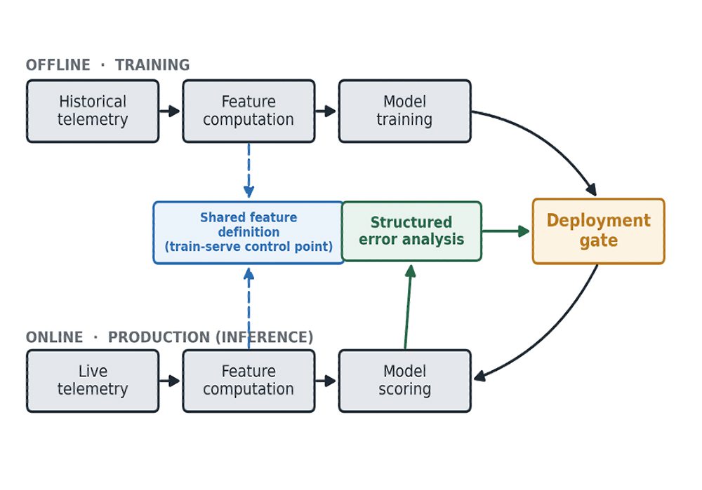
_{Figure 1. Validation architecture. Features are defined once and consumed by both the training and inference paths (the train-serve control point). Model scoring feeds structured error analysis, whose results decide whether a model clears the deployment gate.}

Conclusions:

If a model reports a quantity over a horizon longer than the observed data, part is measurement and part is assumption—report the split, test against several tail assumptions, and decline horizons where extrapolation dominates. That omission matters because the two parts carry very different risk: a precise-looking figure can be almost entirely assumption, and any decision anchored to it—capital planning, replacement schedules, contractual commitments—inherits a fragility nobody has accounted for. Reporting the split is the difference between acting on evidence and acting on a guess wearing a decimal point.

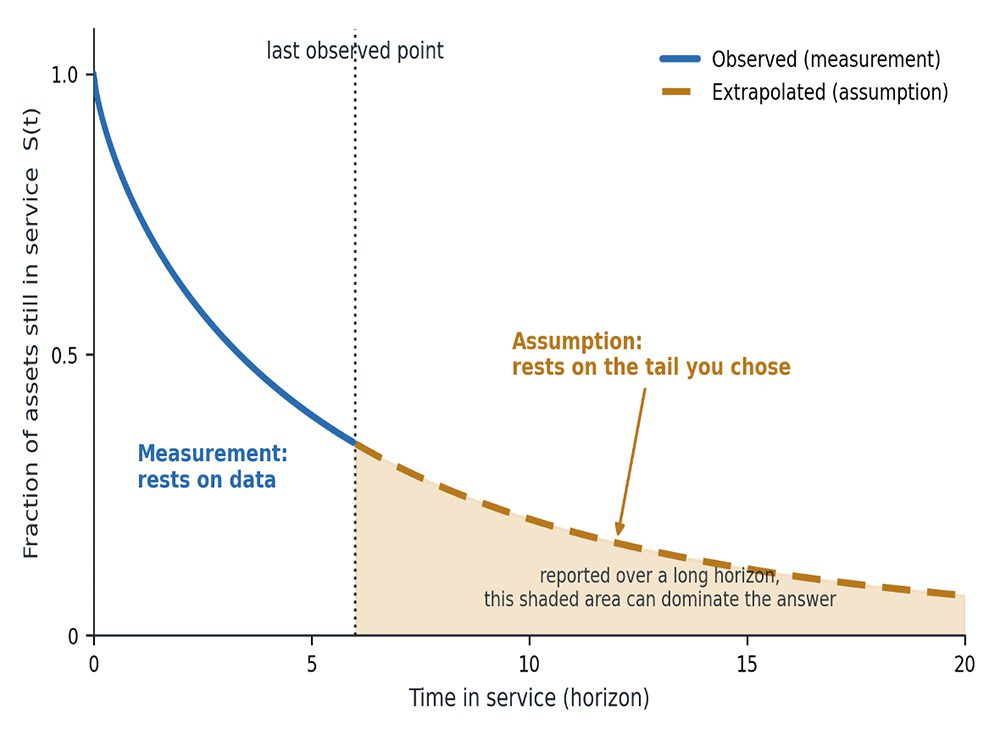
_{Figure 2. Reporting beyond the observed window, shown for an equipment time-to-failure (survival) model. Up to the last observed point the fraction of assets still in service rests on data (solid); beyond it, the curve rests on a chosen tail assumption (dashed). When such a model reports remaining useful life over a long horizon, the assumed portion can dominate the reported number.}

Second, validation expires: because of drift, a model is only validated as of a date. Repeat the error analysis on a fixed cadence against recent data, compare segment-level results to baseline, and give every deployed model a named owner, a review date, and documented dependencies [10], [11]. The absence of a decommissioning plan turns a stale model into a permanent liability.

For telecom operations, where networks are heterogeneous and the consequential cases are usually the rare ones, the recommendation is blunt: require the error map, not the accuracy number, before deployment.

About the Author:

Priyank Jain is a Data Scientist II at Boost Mobile, where he builds production machine learning across retail and telecom, including subscriber survival and churn models, demand and traffic forecasting, and location recommendation systems. He has over seven years in applied machine learning, is an IEEE graduate student member, and has authored peer-reviewed journal and conference papers. LinkedIn: https://www.linkedin.com/in/priyankjn7//

References:

[1] “What is data drift in ML, and how to detect and handle it,” Evidently AI, Jan. 9, 2025. [Online]. Available: https://www.evidentlyai.com/ml-in-production/data-drift

[2] “What is data drift in machine learning,” Chalk AI, Apr. 9, 2026. [Online]. Available: https://chalk.ai/blog/data-drift

[3] “Concept drift,” Wikipedia. [Online]. Available: https://en.wikipedia.org/wiki/Concept_drift

[4] “Survival analysis and interpretation of time-to-event data,” PMC/NIH, Jul. 13, 2018. [Online]. Available: https://pmc.ncbi.nlm.nih.gov/articles/PMC6110618/

[5] “Survival analysis,” Wikipedia. [Online]. Available: https://en.wikipedia.org/wiki/Survival_analysis

[6] “Measuring Goodhart’s law,” OpenAI, Apr. 13, 2022. [Online]. Available: https://openai.com/index/measuring-goodharts-law/

[7] “On Goodhart’s law, with an application to value alignment,” arXiv:2410.09638, Oct. 12, 2024.

[8] “Class-imbalanced datasets,” Google Machine Learning Crash Course. [Online]. Available: https://developers.google.com/machine-learning/crash-course/overfitting/imbalanced-datasets

[9] “5 effective ways to handle imbalanced data in machine learning,” MachineLearningMastery, Apr. 20, 2025. [Online]. Available: https://machinelearningmastery.com/5-effective-ways-to-handle-imbalanced-data-in-machine-learning/

[10] “MLOps: Continuous delivery and automation pipelines in machine learning,” Google Cloud, Aug. 28, 2024. [Online]. Available: https://docs.cloud.google.com/architecture/mlops-continuous-delivery-and-automation-pipelines-in-machine-learning

[11] “MLOps lifecycle: Stages, workflow, and best practices,” LaunchDarkly, May 30, 2026. [Online]. Available: This entry was posted in Uncategorized. Bookmark the permalink.